3차원 회전 행렬과 각속도

3차원 회전 행렬을 미분하여 각속도 벡터를 유도해 보자

앞서서 2차원 회전 행렬과 각속도의 관계를 행렬의 미분을 통해 알아보았다.

그렇다면 3차원 역시도 회전 행렬을 미분하여 각속도 벡터를 유도할 수 있는가?
된다면 그 관계는 어떻게 될 것인가.

행렬곱의 미분

유도에 앞서, 먼저 짚고 넘어가야할 점은 행렬곱의 미분이다.

말은 어렵게 했지만 수식으로 보면 오히려 간단하다.

2개의 행렬 $A,B$가 있을 때, 다음을 생각해 보는 것이다.

\[\begin{align} \frac{d}{dt}\left(A B\right) = ? \end{align}\]

결론부터 먼저 말하자면 다음과 같다

\[\begin{align} \frac{d}{dt}\left(AB \right) &= \dot{A}B + A\dot{B} \\ \nonumber \\ \text{if } A &= \begin{bmatrix} a_{11} & \cdots & a_{1m} \\ \vdots & \ddots & \vdots \\ a_{n1} & \cdots & a_{nm} \end{bmatrix},\nonumber \\[10pt] \frac{dA}{dt} = \dot{A} &= \begin{bmatrix} \dot{a_{11}} & \cdots & \dot{a_{1m}} \\ \vdots & \ddots & \vdots \\ \dot{a_{n1}} & \cdots & \dot{a_{nm}} \end{bmatrix} \end{align}\]

이제 어떻게 저런 결과가 나올 수 있는지 생각해 보자.

보통 $A_{n \times m}$은 $n$행 $m$열을 가진 행렬 $A$를 말한다.
다음의 행렬을 생각해 보자

\[\begin{align} A_{n \times m}, B_{m \times p}, \nonumber\\ AB = C_{n \times p} \nonumber \end{align}\]

이를 실제 행렬 형태로 나타내면 다음과 같다

\[\begin{align} A_{n \times m} &= \begin{bmatrix} a_{11} & a_{12} & \cdots & a_{1m} \\ a_{21} & a_{22} & \cdots & a_{2m} \\ \vdots & \vdots & \ddots & \vdots \\ a_{n1} & a_{n2} & \cdots & a_{nm} \end{bmatrix} \nonumber \\[10pt] B_{m \times p} &= \begin{bmatrix} b_{11} & b_{12} & \cdots & b_{1p} \\ b_{21} & b_{22} & \cdots & b_{2p} \\ \vdots & \vdots & \ddots & \vdots \\ b_{m1} & b_{m2} & \cdots & b_{mp}, \end{bmatrix} \nonumber\\[8pt] C_{n \times p} &= A_{n \times m} B_{m \times p} \nonumber \\ \nonumber \\ \begin{bmatrix} c_{11} & c_{12} & \cdots & c_{1p} \\ c_{21} & c_{22} & \cdots & c_{2p} \\ \vdots & \vdots & \ddots & \vdots \\ c_{n1} & c_{n2} & \cdots & c_{np} \end{bmatrix} &= \begin{bmatrix} a_{11} & a_{12} & \cdots & a_{1m} \\ a_{21} & a_{22} & \cdots & a_{2m} \\ \vdots & \vdots & \ddots & \vdots \\ a_{n1} & a_{n2} & \cdots & a_{nm} \end{bmatrix} \begin{bmatrix} b_{11} & b_{12} & \cdots & b_{1p} \\ b_{21} & b_{22} & \cdots & b_{2p} \\ \vdots & \vdots & \ddots & \vdots \\ b_{m1} & b_{m2} & \cdots & b_{mp}, \end{bmatrix} \label{e1} \end{align}\]

위 식 $\eqref{e1}$ 에서 행렬 $C$의 원소, $c_{ij}$가 어떻게 계산되는지를 살펴보면 다음과 같다.

\[\begin{align} c_{11} &= a_{11}b_{11} + a_{12}b_{21} + \cdots + a_{1m}b_{m1} \nonumber \\ c_{12} &= a_{11}b_{12} + a_{12}b_{22} + \cdots + a_{1m}b_{m2} \nonumber \\ c_{21} &= a_{21}b_{11} + a_{22}b_{21} + \cdots + a_{2m}b_{m1} \nonumber \\ \vdots \nonumber \\ \therefore c_{ij} &= \sum_{k=1}^{m}a_{ik} b_{kj} \label{e2} \end{align}\]

이제, 식 $\eqref{e1}, \eqref{e2}$를 사용하여 정리하면 우리가 원하는 결과가 나온다.

\[\begin{align} \text{from } \frac{d}{dt}C, \nonumber \\ \dot{c_{ij}} &= \sum_{k=1}^{m}\left(\dot{a_{ik}}b_{kj} + a_{ik}\dot{b_{kj}} \right) \nonumber \\ &= \sum_{k=1}^{m}\dot{a_{ik}}b_{kj} + \sum_{k=1}^{m}a_{ik}\dot{b_{kj}} \nonumber \\ \nonumber \\ \therefore \dot{C} &= \frac{d}{dt}\left(AB\right) = \dot{A}B + A\dot{B} \end{align}\]

조금 더 생각해 보면, 3개나 그 이상의 행렬곱의 미분도 알아차릴 수 있다.
기존의 스칼라의 곱을 미분할 때와 다를바가 없다.

\[\begin{align} \frac{d}{dt}\left(ABC\right) &= \frac{d(AB)}{dt}C + (AB)\frac{dC}{dt} \nonumber \\[8pt] &= \left(\dot{A}B + A\dot{B} \right)C + (AB)\dot{C} \nonumber \\[8pt] &= \dot{A}BC + A\dot{B}C + AB\dot{C} \end{align}\]

회전 변환의 미분과 각속도 벡터

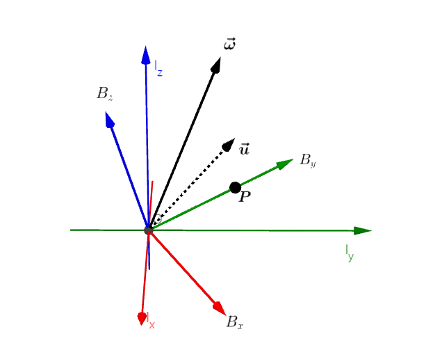그림 1 : 벡터 u로 회전된 좌표계 B와 각속도 벡터

그림1 에서 회전하는 좌표계 $B$와 $B$에 붙어서 움직이는 점 $P$를 생각해보자.

좌표계 $I$에 상대적으로 좌표계 $B$가 현재 회전된 정도를 회전 행렬 $R$로 표현했다고 하자. 이는 $B$의 각각의 축 벡터를 행으로 가지는 $3 \times 3$ 행렬이 될 것이다.

$I$에 상대적으로 $B$가 회전중일 때, 그 각속도 벡터를 $\omega$라 하자.
$\omega_I, \omega_B$는 각속도 벡터 $\omega$를 각각 좌표계 $I$와 $B$에서 관찰했을 때의 벡터값이다. 3차원에서는 각속도도 벡터이므로, 관찰하는 좌표계에 따라서 각속도 벡터의 표현도 달라진다.

$P_{I}, P_{B}$역시도 각각 $I, B$ 에서 점 $P$를 관찰했을 때의 좌표라고 생각하자.
$B$의 입장에서 점 $P$의 위치는 움직이지 않지만, $I$에서 봤을 때는 $B$가 각속도 $\omega$로 회전하고 있기 때문에, 시간에 대해 변하는 위치가 된다.

따라서 다음이 성립한다. \(\begin{align} \frac{d}{dt}P_I \neq 0 \\[8pt] \frac{d}{dt}P_B = 0 \\[8pt] RP_B = P_I \label{e3} \end{align}\)

이제 $\eqref{e3}$의 양변을 미분하면, 각속도와의 관계를 알 수 있다.

\[\begin{align} \frac{d}{dt}\left( R P_B \right) &= \frac{d}{dt} P_I \nonumber \\ \dot{R}P_B &= V_I = [\omega_I]_\times P_I \label{e4} \\ &= [\omega_I]_\times R P_B, P_B \in \mathbb{R}^3 \nonumber \\ \nonumber \\ \therefore \dot{R} &= [\omega_I]_\times R \nonumber \\ => \dot{R}R^T &= [\omega_I]_\times = \begin{bmatrix} 0 & -\omega_{zI} & \omega_{yI} \\ \omega_{zI} & 0 & -\omega_{xI} \\ -\omega_{yI} & \omega_{xI} & 0 \end{bmatrix} \label{e5} \end{align}\]

식 $\eqref{e4}$ 부분은 동역학에서 회전하는 관성계의 운동에 대한 부분 중, 상대속도에 대한 내용이다. 다음을 참고하자.

참고1 : Rotating Reference Frame
참고2 : 회전하는 좌표계에서 운동하는 물체의 속도와 가속도

Body Rate 벡터와의 관계

Body Rate는 그냥 이미 위에서 정의한 $\omega_B$ 벡터를 별도로 부르는 말이다.

왜 괜히 따로 용어가 붙었는지 불만일 수 있다. 하지만 이건 $\omega_I$ 보다 $\omega_B$를 더 많이 쓰기 때문이다.
비행체의 3차원 자세 제어 등의 실전에서는 아무도 $\omega_I$ 벡터엔 관심이 없다. 이유는 더 많지만 일부분을 소개하자면 다음과 같다.

• 보통 비행체의 몸체에 아예 추진력을 내는 장치가 달려있으므로, Body Frame ($B$ 좌표계)로 벡터들을 통일하는 것이 훨씬 편하다.
• 강체의 Net Torque는 3차원의 경우, $\tau = I\alpha + \omega \times(I\omega)$로 표현된다.
  이때 각각의 $I$(질량관성모멘트 텐서), $\alpha$(각가속도), $\omega$(각속도) 벡터를 관찰하는 좌표계가 통일되어 있기만 하면 등식이 성립한다.

  참고 : Euler’s equations (rigid body dynamics)

• 이때, 회전하는 물체의 질량관성모멘트 텐서$I$는 기준계에서 관찰할 땐 시간에 대해 변하지만, body frame에서 관찰할 땐 그 값이 시간에 따라 변하지 않는다.
  즉 미분할 때 깔끔하며, 측정을 통해 알아낸 값을 사용해서 모델 기반 제어에 사용할 수도 있다.

이제 위의 식 $\eqref{e5}$를 조금 변형하여 $\omega_B$로 만들 텐데, 그 전에 알고 가야할 성질이 하나 있다.

\[\begin{align} \text{let }R \text{ is Rotation Matrix in 3D}, \nonumber \\ \text{if }\vec{c} &= \vec{a} \times \vec{b}, \nonumber \\ R\vec{c} &= (R\vec{a}) \times (R\vec{b}) \label{e6} \\ \nonumber \\ \therefore c &= [a]_\times b \nonumber \\ => Rc &= [Ra]_\times Rb \label{e7} \end{align}\]

식 $\eqref{e6}$가 가능한 이유는 회전 변환이 길이를 유지하고, 변환 후의 두 벡터 사이의 각도 역시 유지하는 성질을 가졌기 때문이다.

이제 $\eqref{e5}, \eqref{e7}$를 조합하면 $\omega_B$에 대한 관계로 바꿀 수 있는데,
다음과 같다.

\[\begin{align} \dot{R}&= [\omega_I]_\times R \nonumber \\ => R^T\dot{R} &= [R^T \omega_I]_\times (R^T R) \nonumber \\ \nonumber \\ \therefore R^T \dot{R} &= [\omega_B]_\times \end{align}\]

지금까지의 결과를 정리해보자.

3차원 회전 행렬 $R$과, 기준계 $I$, 강체의 좌표계 $B$, $I$에 상대적인 $B$의 각속도 벡터를 $\omega$,
$I$와$B$에서 관찰한 $\omega$를 각각 $\omega_I, \omega_B$라 했을 때,

\[\begin{align} \dot{R}R^T = [\omega_I]_\times \\ R^T \dot{R} = [\omega_B]_\times \end{align}\]

$[]_\times$는 벡터의 Cross Product Matrix이며, 다음과 같다.

\[\begin{align} \vec{a} = (a_x, a_y, a_z) \\ [a]_\times = \begin{bmatrix} 0 & -a_z & a_y \\ a_z & 0 & -a_x \\ -a_y & a_x & 0 \end{bmatrix} \end{align}\]

참고 : Cross_product(Conversion to matrix multiplication)

2차원 회전과 각속도 revisit

포스트 각도 표현의 미분 불가능 문제와 복소수 - 회전 행렬은 미분 가능한가?에서 유도한 2차 회전 행렬과 각속도 값의 관계는 다음과 같다.

\[\begin{align} \text{let } R \text{ : 2D rotation matrix}, \nonumber \\ R(\theta) &= \begin{bmatrix} \cos{\theta} & -\sin{\theta} \\ \sin{\theta} & \cos{\theta} \end{bmatrix} \nonumber \\ \nonumber \\ \dot{R} \begin{bmatrix} -\sin{\theta} & \cos{\theta} \\ -\cos{\theta} & -\sin{\theta} \end{bmatrix} &= \dot{\theta}I \label{e8} \end{align}\]

이제 식 $\eqref{e5}$를 변형하여 $\eqref{e8}$를 만들어 보자.
3차원의 회전 중에서, xy 평면에 대한 회전으로 해석 해보면 다음과 같다.

\[\begin{align} R_3 &= \begin{bmatrix}R(\theta) & 0 \\ 0 & 1 \end{bmatrix} \nonumber \\[8pt] \omega_I &= \begin{bmatrix} 0 & 0 & \dot{\theta} \end{bmatrix}^T \nonumber \\ \nonumber \\ \dot{R_3}R_3^T &= [\omega_I]_\times = \begin{bmatrix} 0 & -\dot{\theta} & 0 \\ \dot{\theta} & 0 & 0 \\ 0 & 0 & 0 \end{bmatrix} \nonumber \\ \nonumber \\ => \dot{R(\theta)} R(\theta)^T &= \dot{\theta}\begin{bmatrix}0 & -1 \\ 1 & 0\end{bmatrix} \nonumber \\[8pt] => \dot{R(\theta)} \begin{bmatrix} \cos{\theta} & \sin{\theta} \\ -\sin{\theta} & \cos{\theta} \end{bmatrix} &= \dot{\theta}\begin{bmatrix}0 & -1 \\ 1 & 0\end{bmatrix} \nonumber \\[8pt] => \dot{R(\theta)} \begin{bmatrix} \cos{\theta} & -\sin{\theta} \\ -\sin{\theta} & -\cos{\theta} \end{bmatrix} &= \dot{\theta}\begin{bmatrix}0 & 1 \\ 1 & 0\end{bmatrix} \nonumber \\[8pt] => \dot{R(\theta)} \begin{bmatrix} -\sin{\theta} & \cos{\theta} \\ -\cos{\theta} & -\sin{\theta} \end{bmatrix} &= \dot{\theta}\begin{bmatrix}1 & 0 \\ 0 & 1\end{bmatrix} = \dot{\theta}I \label{e9} \\ \end{align}\]

이렇게 식 $\eqref{e8}$과 $\eqref{e9}$가 완전히 동일한 결과가 나오는 것을 확인할 수 있다.

3차원의 회전 변환은 2차원 회전 변환의 확장판인 만큼, 2차원 회전 변환에서 유도되는 모든 성질들을 이끌어낼 수 있다.

다음 포스트부터는 본격적으로 3차원 회전에 대한 내용을 시작하도록 하겠다.